Overview
The project afforded an inside look into something that has fascinated me for a very long time--real-time cloth simulation.
Using a mass and spring model, we were able to simulate cloth movement over time due to internal and external forces.
To enhance realism, we then looked at collisions with other objects and self-collision to prevent cloth clipping and
other unnatural behavior. Finally, we implemented a number of GLSL shaders: diffuse, Blinn-Phong,
texture mapping, bump mapping, displacement mapping, and mirror. Overall, this project was one of my favorites--as much as
I enjoy waiting for images to render, being able to the cloth drape over the sphere in real-time made for some very
awe-inspiring moments. It's amazing to me that a simple mass and spring model can approximate the real world so closely.
Part I: Masses and springs
We began by modelling the cloth as a grid of point masses and springs.
Specifically, the grid consists of
num_width_points by
num_height_points
masses spanning
width and
height, respectively. If the cloth is orientated
horizontally, the
y coordinate is set to 1, and the points vary along the
xz
plane; otherwise, the
z coordinate is chosen randomly in the range -1/1000 and 1/1000,
and the masses vary along the
xy plane. If applicable, in addition to its location
specification, the mass is also marked as pinned.
To apply the structural, shear, and bending constraints, we create springs between pairs of masses
as follows:
- Structural: Between a mass and its left neighbor and top neighbor.
- Shearing: Between a mass and its neighbor to the upper right and upper left.
- Bending: Between a mass and its neighbor two to the left and two above.
Screenshots
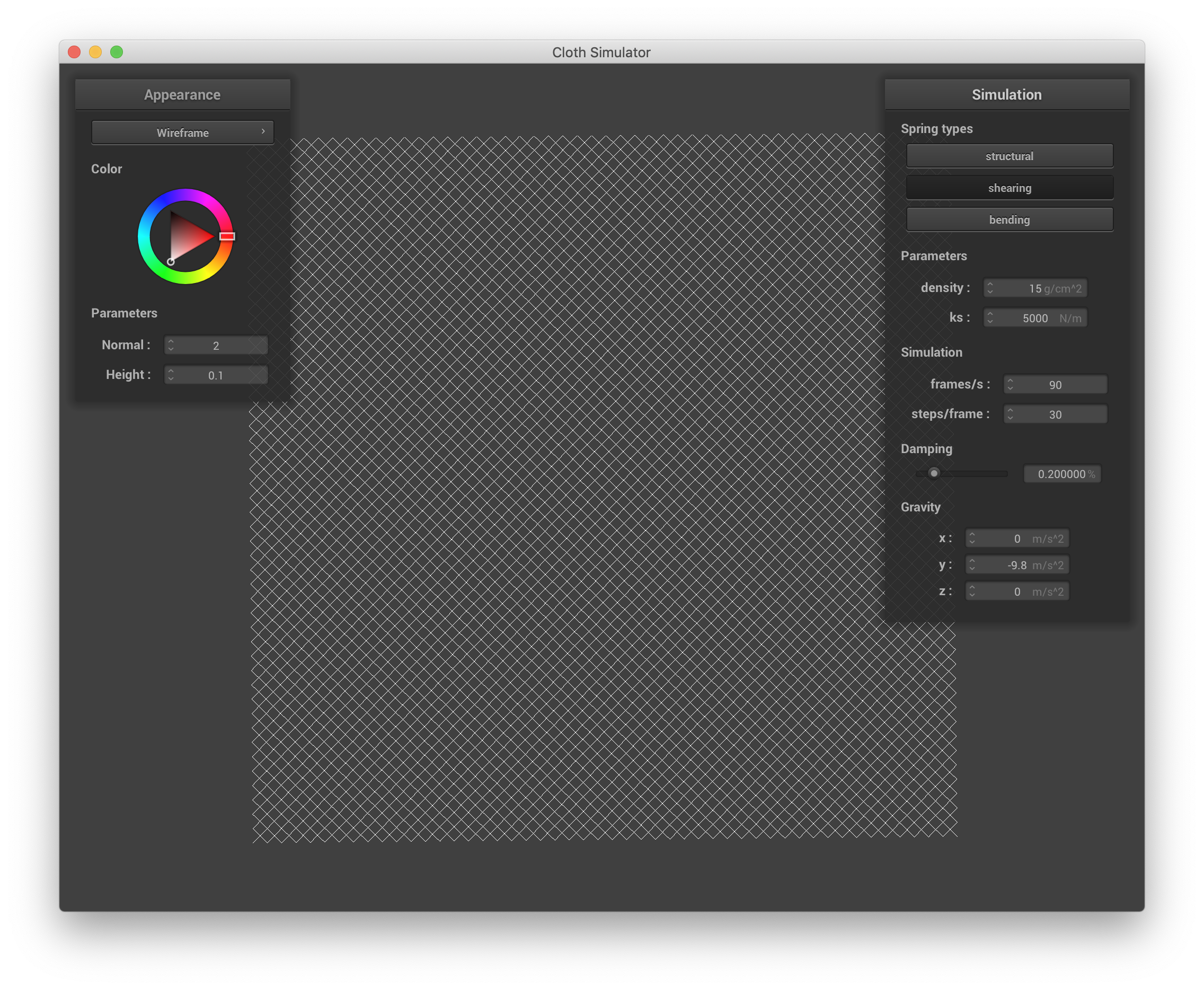
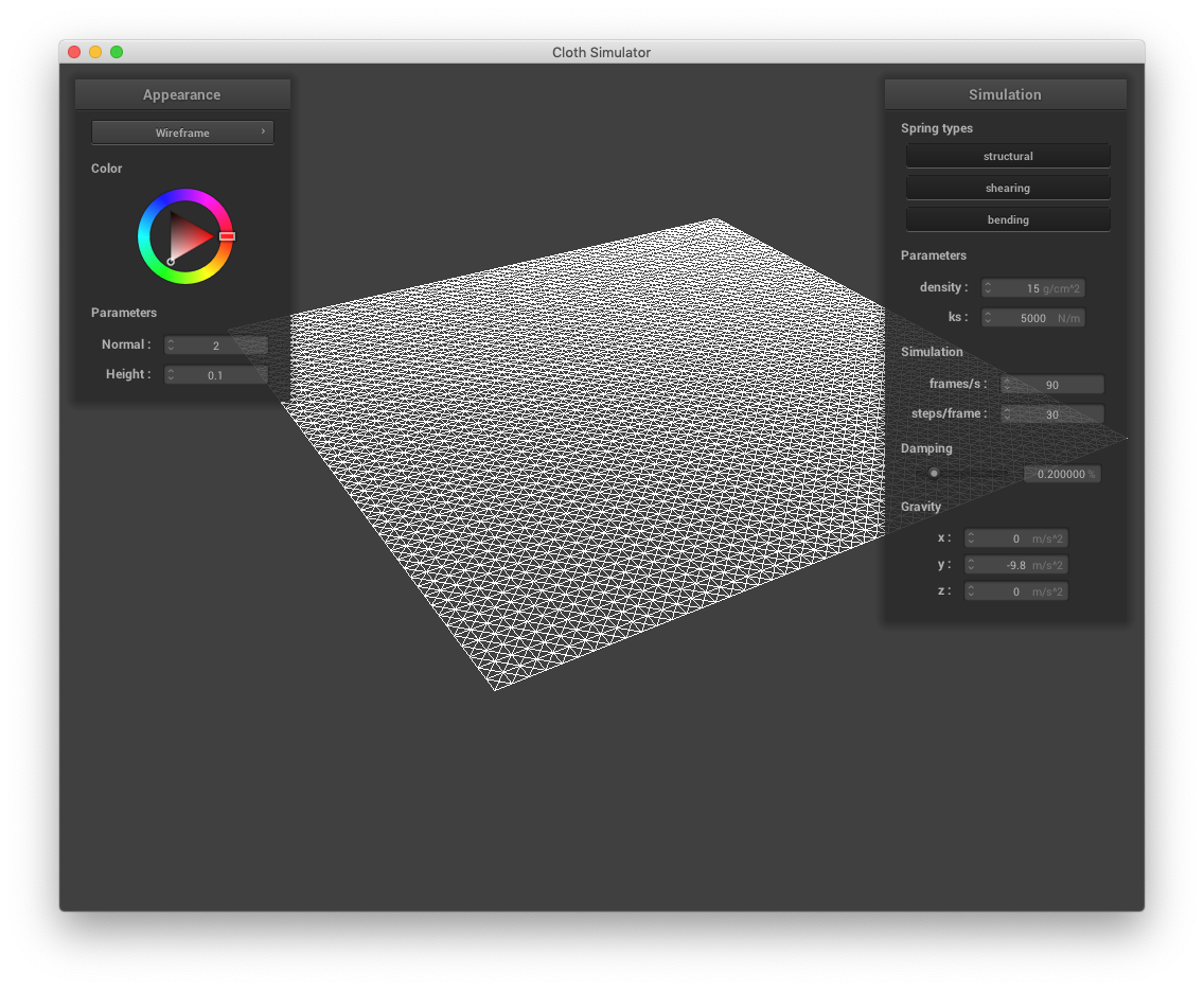 Wireframe structure
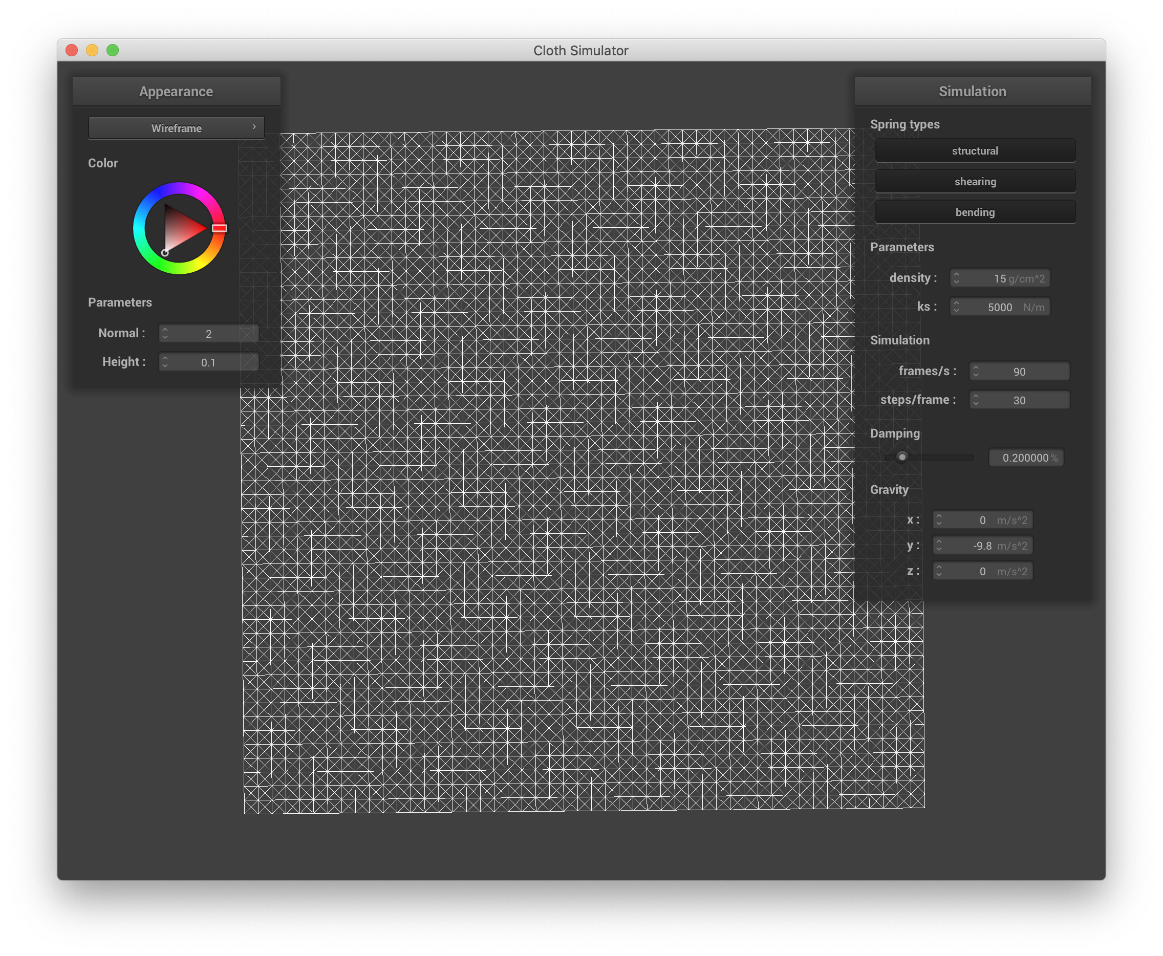 Wireframe with all constraints
 Wireframe with only shearing
 Wireframe with no shearing
Part II: Simulation via numerical integration
With the model now built, we can now simulate the cloth's motion using the physical equations
that govern point masses and springs. Specifically, taking into account all the forces acting on each
point mass at each time step, we can compute the dynamic shape and location of the cloth.
The simulation process is done in three steps:
-
Force calculation: In addition to the forces applied by external acceleration, we must also
consider the spring correction forces, which can be calculated by:

ks is the spring constant, p_a and p_b
are the point masses' positions, and l is the spring's rest length.
The force vector itself is the vector from one point mass to the other with the magnitude of this
spring correction force.
-
Position calculation: Using Verlet integration, we can calculate the new position of each point mass after
a time step
dt as follows:

where d is the damping term. Note that we do not update any pinned point mass.
-
Constrain position updates: To prevent unreasonable deformation, we constrain the position of any two
point masses to be at most 10% greater than the associated spring's rest length after any time step.
Screenshots
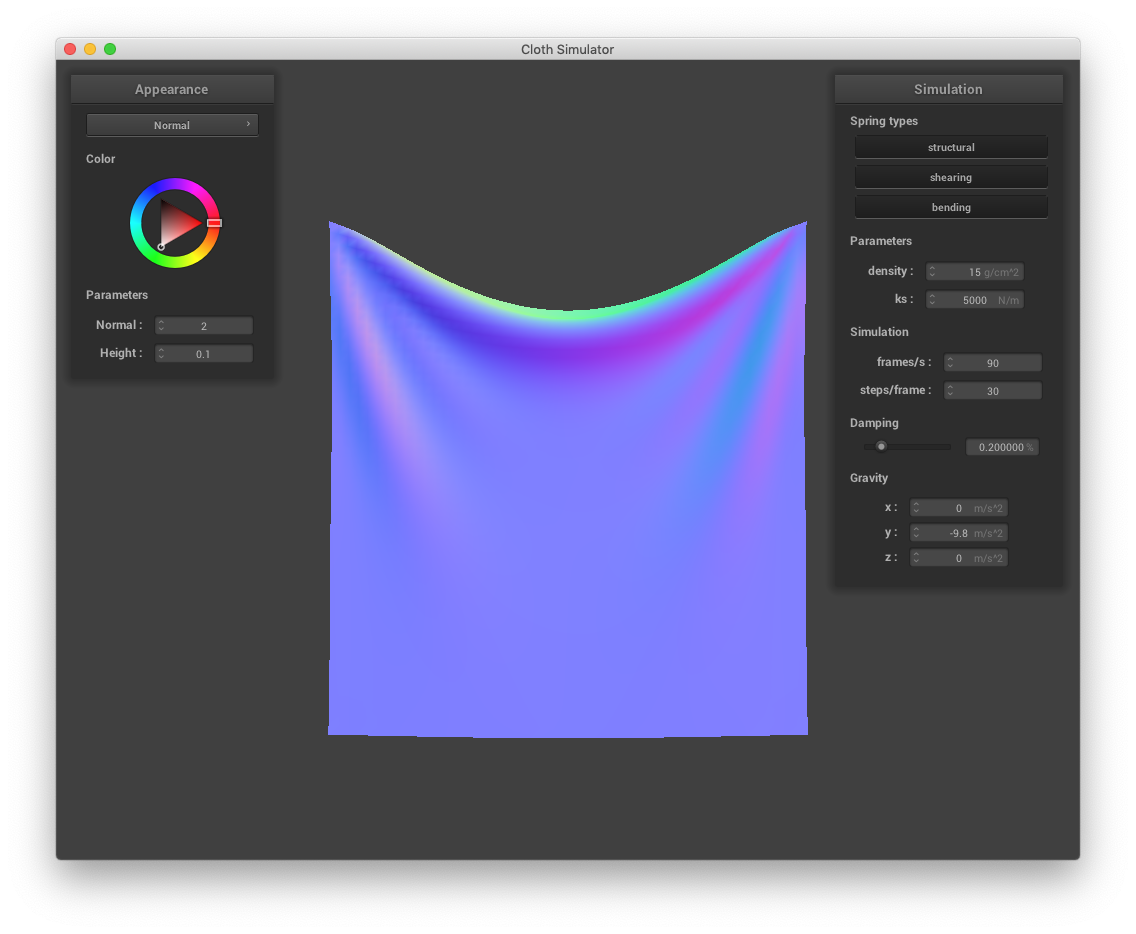
Default Parameters
 Variations in
 ks
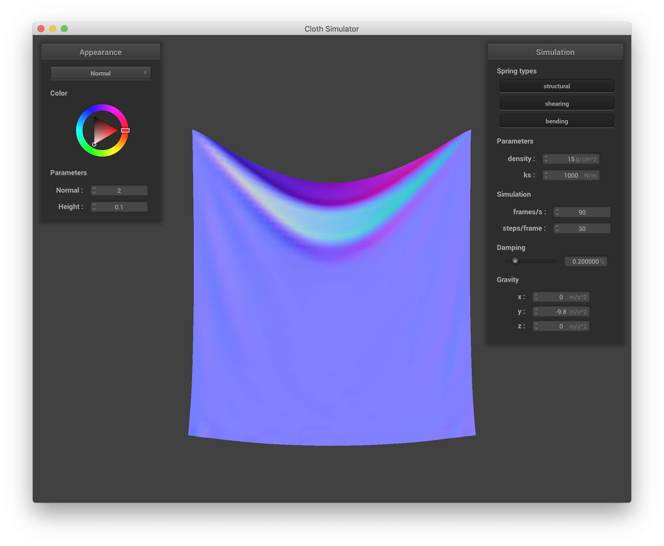 ks of 1000
|
 ks of 10000
|
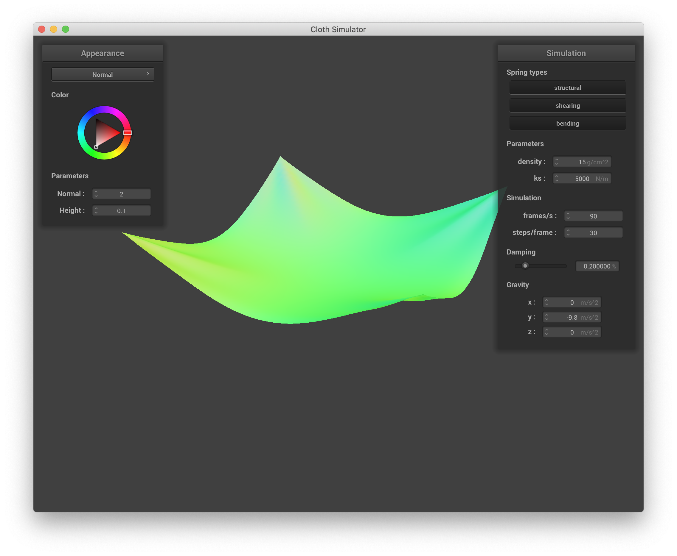
ks is a measure of the spring's stiffness. Notice that in their final resting positions,
the cloth on the left with the lower
ks
contains far more slack (most apparent in the middle droop) than the cloth with default parameters.
In contrast, the cloth on the right with the higher
ks, which
remains closer to its original rectangular shape than both the cloths with low
ks and default parameters.
Variations in density
 Density of 1 g/cm^2
|
 Density of 100 g/cm^2
|
Density is directly proportional to the mass of the cloth. Higher densities result in higher forces, specifically
gravitational,
by Newton's second law. Notice that in their final resting states the cloth on the left with the lower density
seems far less perturbed from its natural state than the cloth with the higher density due to the increase in gravitational force
dragging the latter downwards. The resting place of the cloth with default parameters falls somewhere between them.
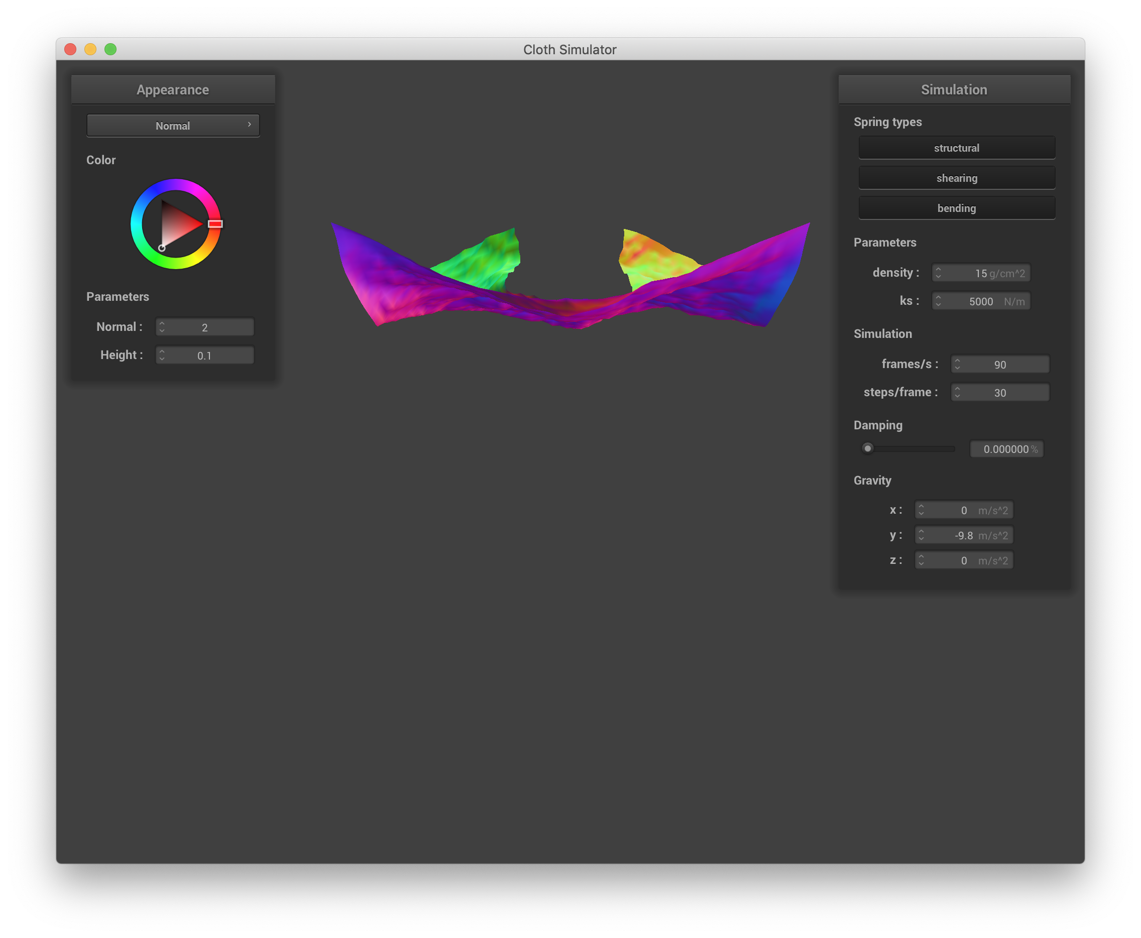
Variations in damping
 Damping of 0%
|
 Damping of 100%
|
The damping term is the catch all for energy lost to friction, heat loss, etc. When it is low, we're essentially conserving
all energy from previous time steps, resulting in a very energetic cloth; whereas when it is high, the cloth's movement is
only dependent on forces from the current time period. Since we do experience energy loss due to air friction in the real world
a larger damping term results in more realistic movement. Notice that the minimal damping on the left results in the cloth
accumulates enough velocity to fling itself horizontally away from the camera shortly after starting the simulation.
In contrast the maximal damping on the left results
in a cloth that reaches equilibrium very quickly. The default cloth falls at a speed somewhere in between the two damping values.
 4 pinned cloth with default settings.
|
Part III: Handling collisions with other objects
To add support for collisions, we added collision detection for primitives in our scenes, specifically spheres and planes. In general,
the idea is to check if a given point mass is inside the primitive--if so, we bump it up to the surface and adjust for friction. We perform
this check for every point mass and every collision object.
For spheres, we do the following:
- Check if the distance from the given point mass to the origin of the sphere is less than the radius.
- If so, compute where the point should have hit the sphere (the tangent point) by extending the path between the current position of the
point mass and the origin of the sphere to the surface of the sphere.
- Compute the correction vector needed to update the point mass's last position to this
new tangent point.
- Add the computed correction vector, scaled by friction, to the point's last position.
For planes, we do the following:
- Check if the sign of the vector formed by the current location of the point mass and a point on the plane dotted with the plane normal
is the same as the sign of the vector formed by the current location of the point mass and a point on the plane dotted with
the vector formed by the previous location of the point mass and a point on the plane.
- If not, compute where the point should have hit the plane (the tangent point) by determining the
intersection of the path between the current position of the
point mass and its previous location with the surface of the plane (e.g., using the
ray and plane collision detection from project 3).
- Compute the correction vector needed to update the point mass's last position to this
new tangent point offset by some surface offset such that the new position remains on the same side of the planeb as
the previous position.
- Add the computed correction vector, scaled by friction, to the point's last position.
Screenshots
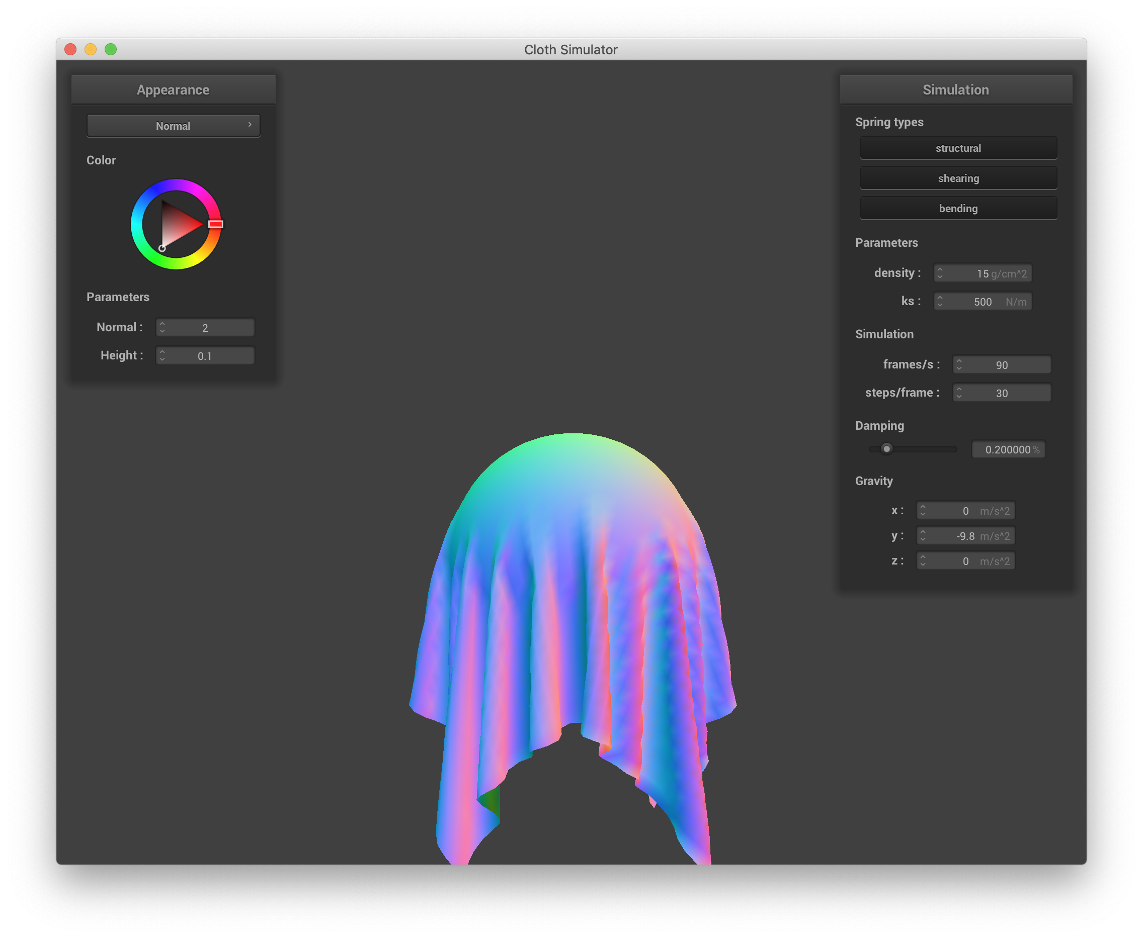
ks of 500
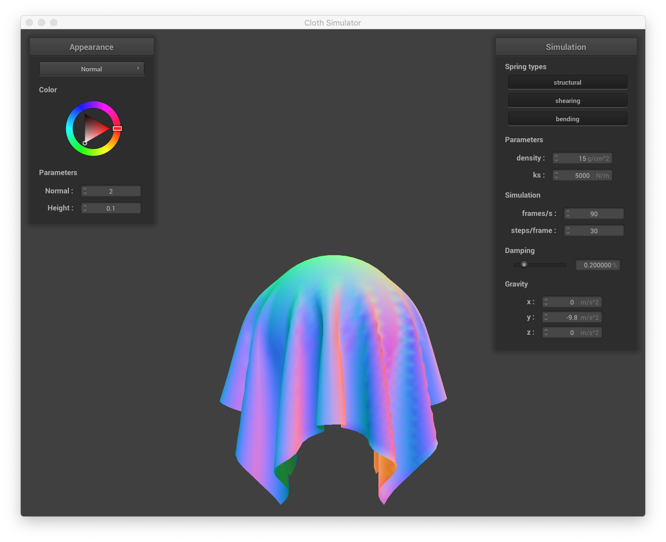
ks of 5000
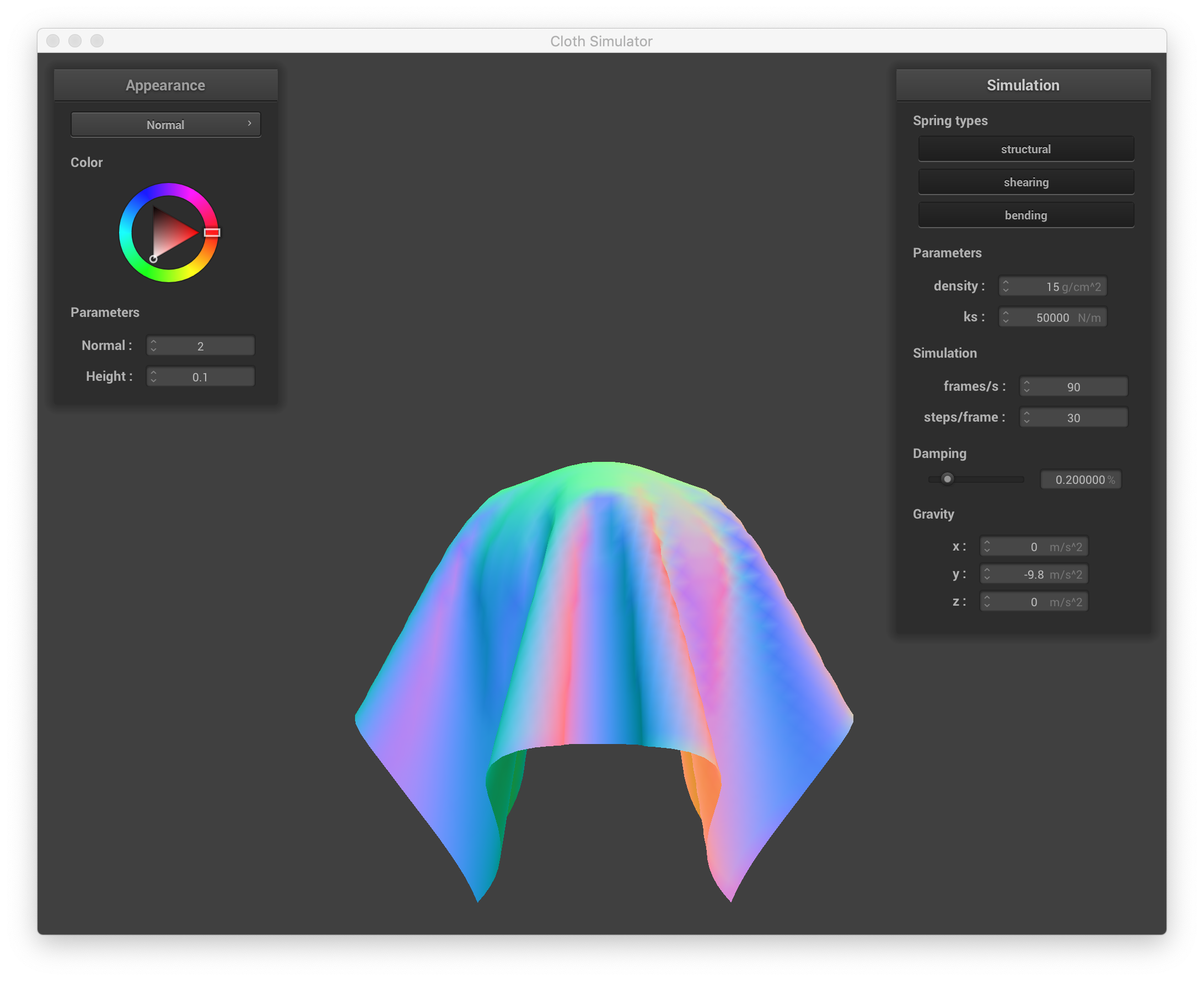
ks of 50000
As noted previously,
ks represents the stiffness of the springs, which effectively controls how strongly the
cloth wants to keep its original rectangular shape. As the value of
ks increases, the less the cloth molds to
the sphere due to excess slack in the springs and the more the cloth tries to retain its rectangular form.
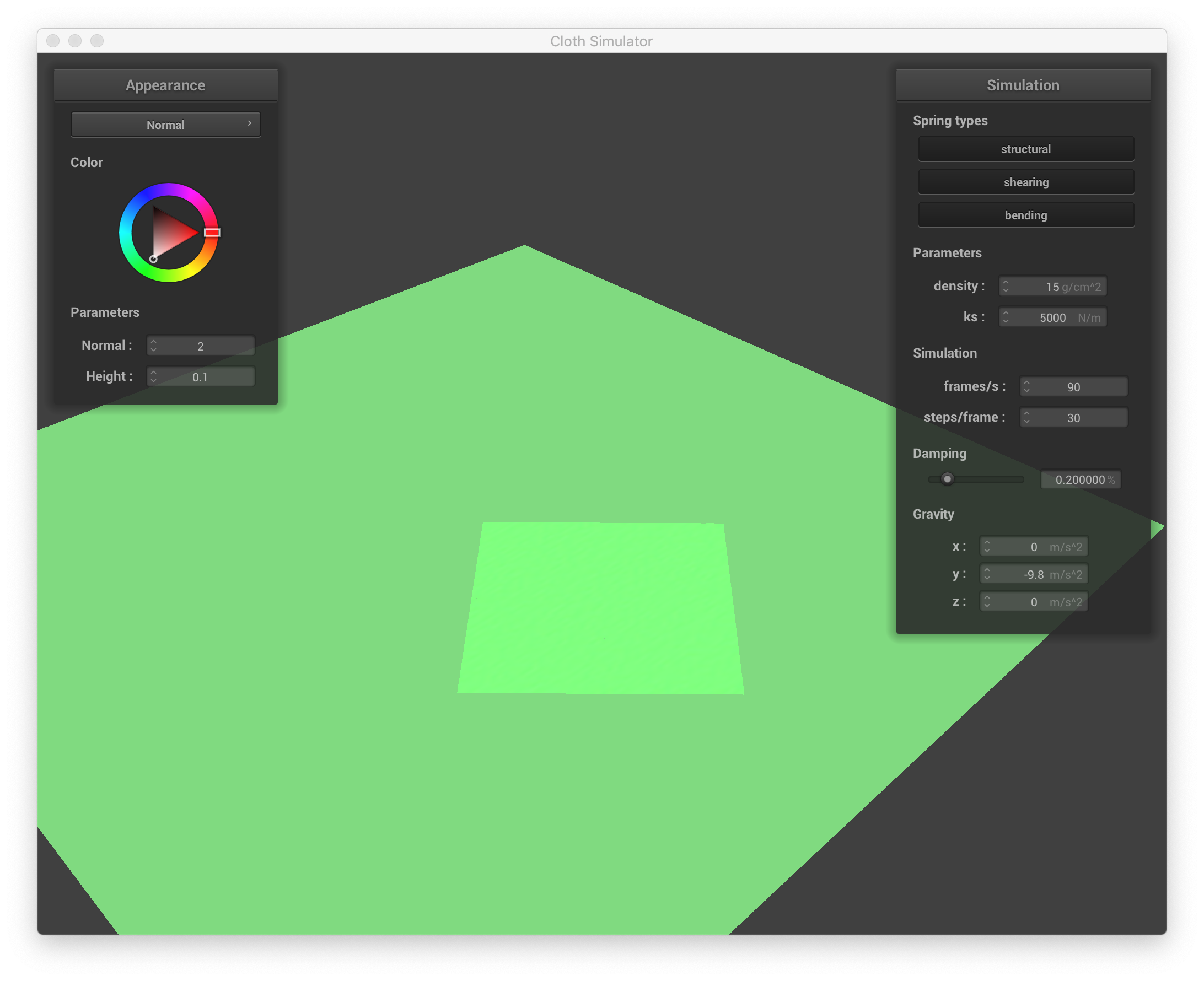
A green cloth lay on a green plane.
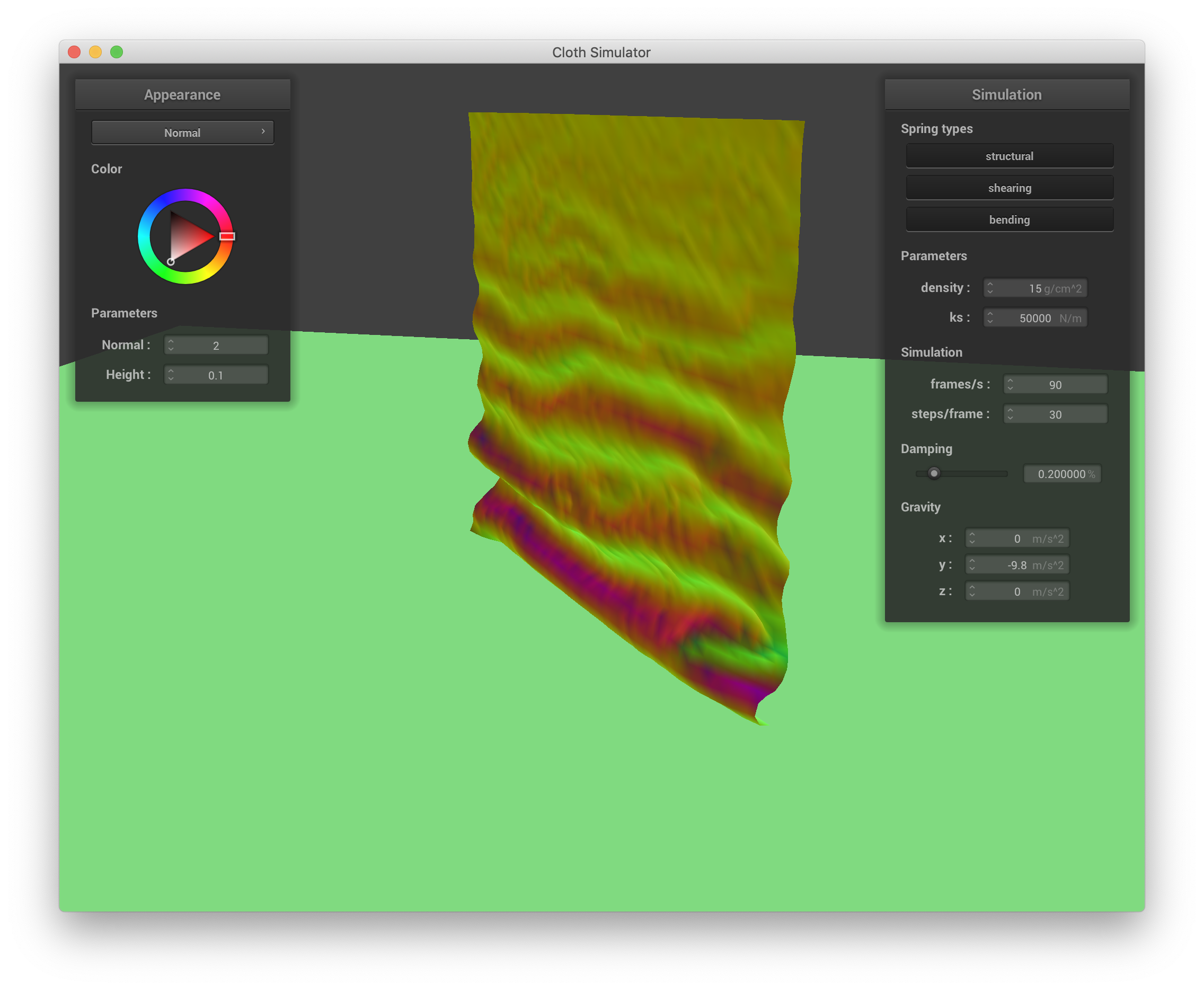
Self Collision Progression
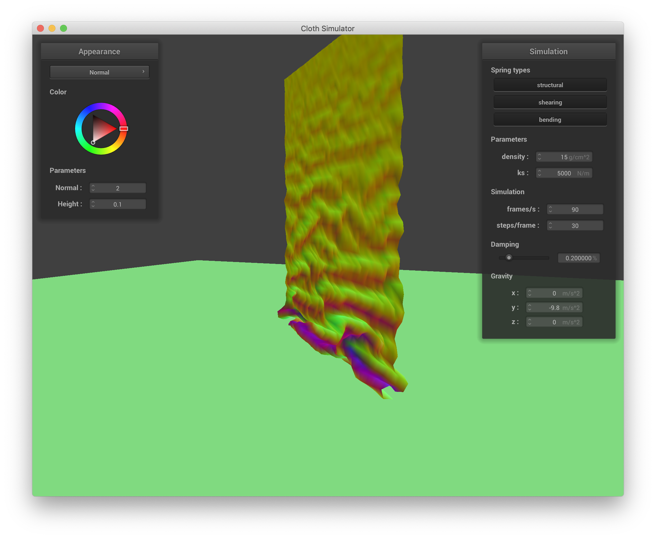 Part 1
|
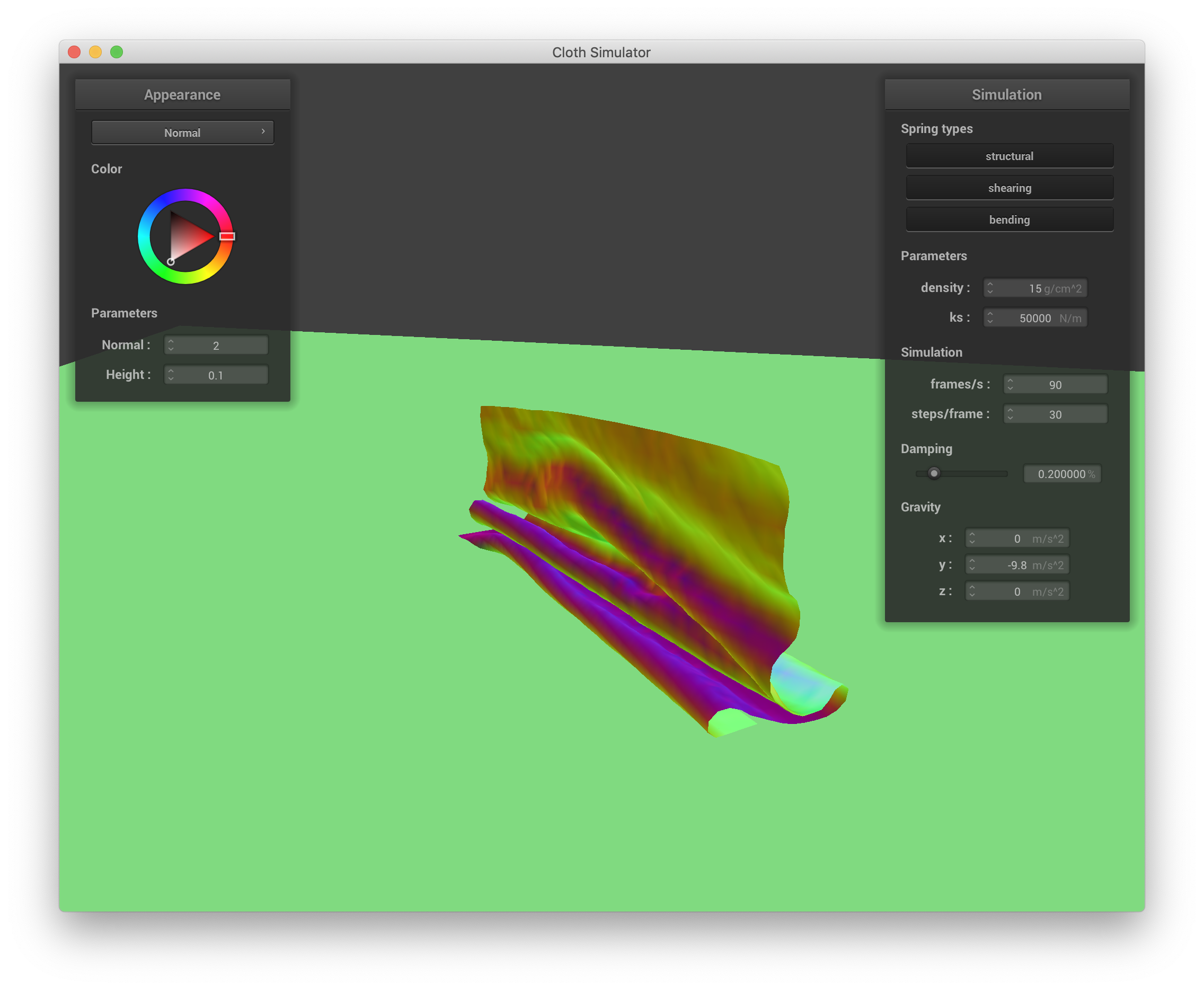
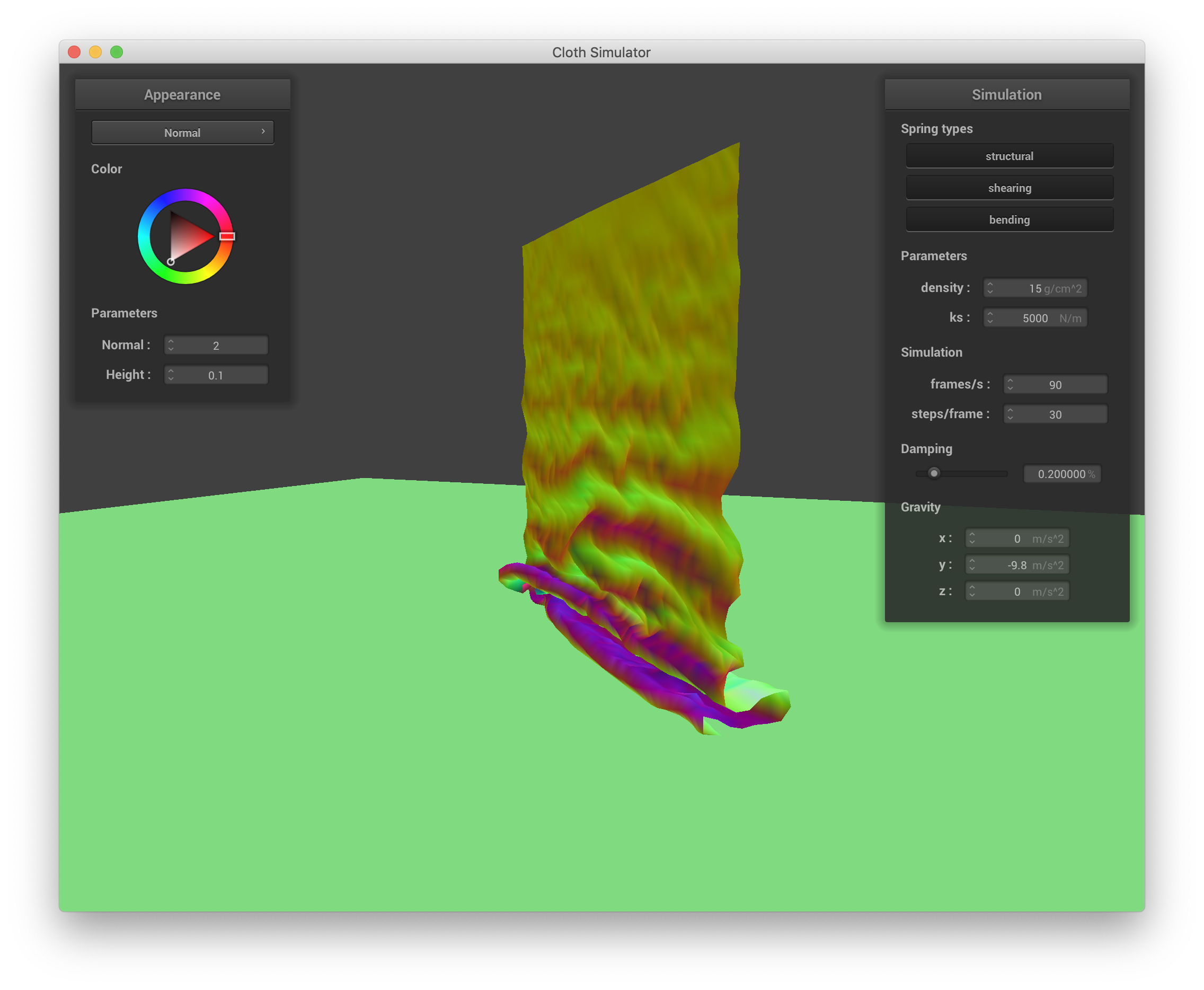 Part 2
|
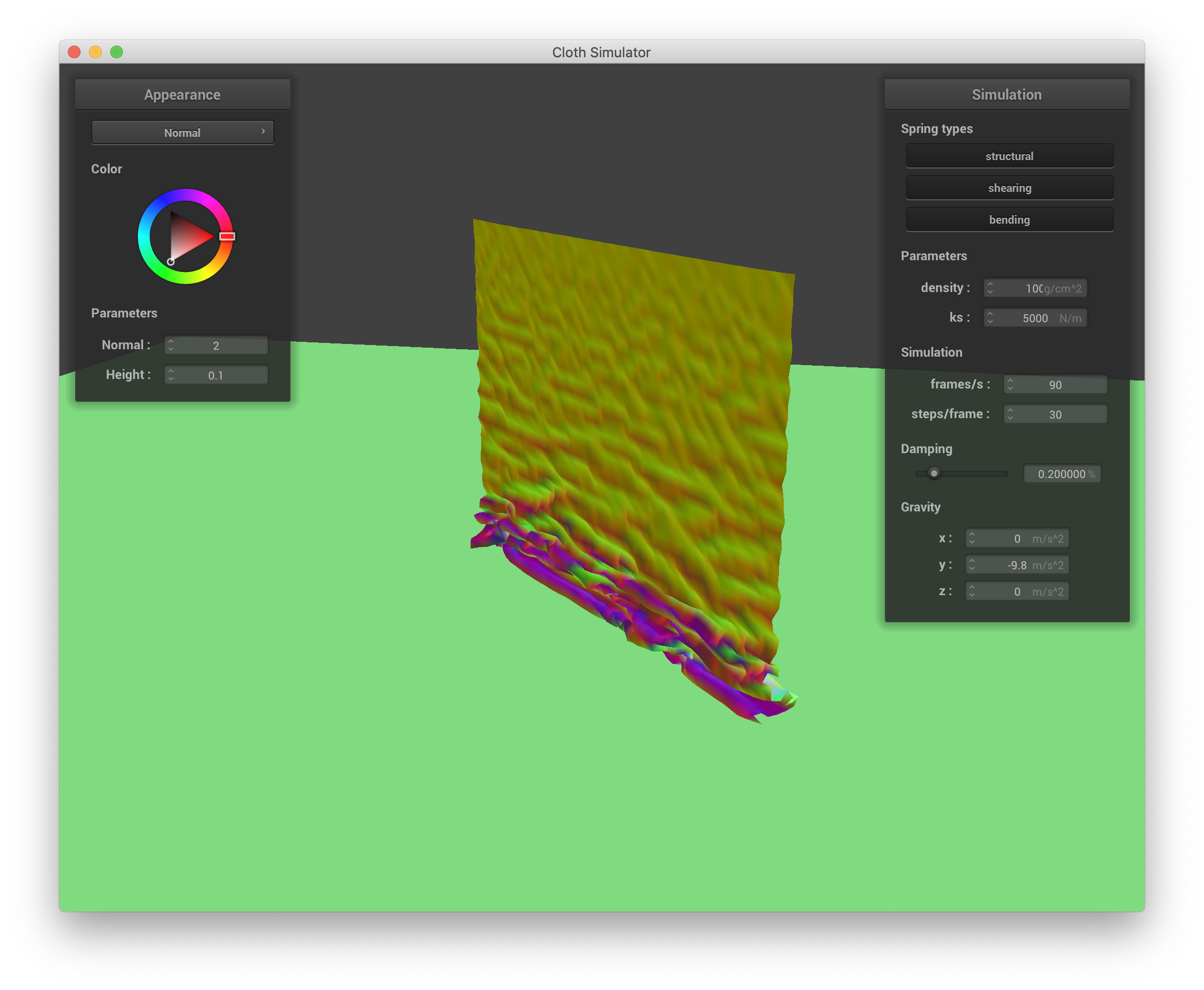
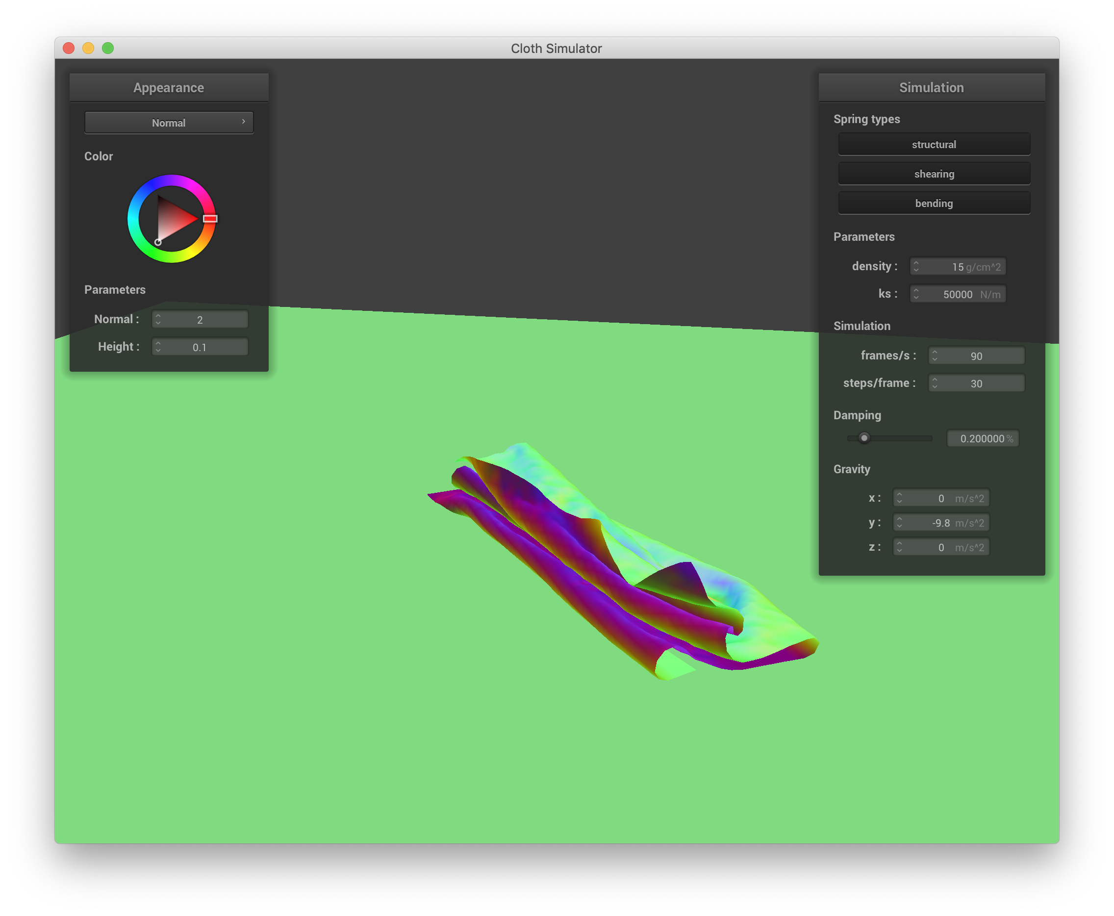
 Part 3
|
 Part 4
|
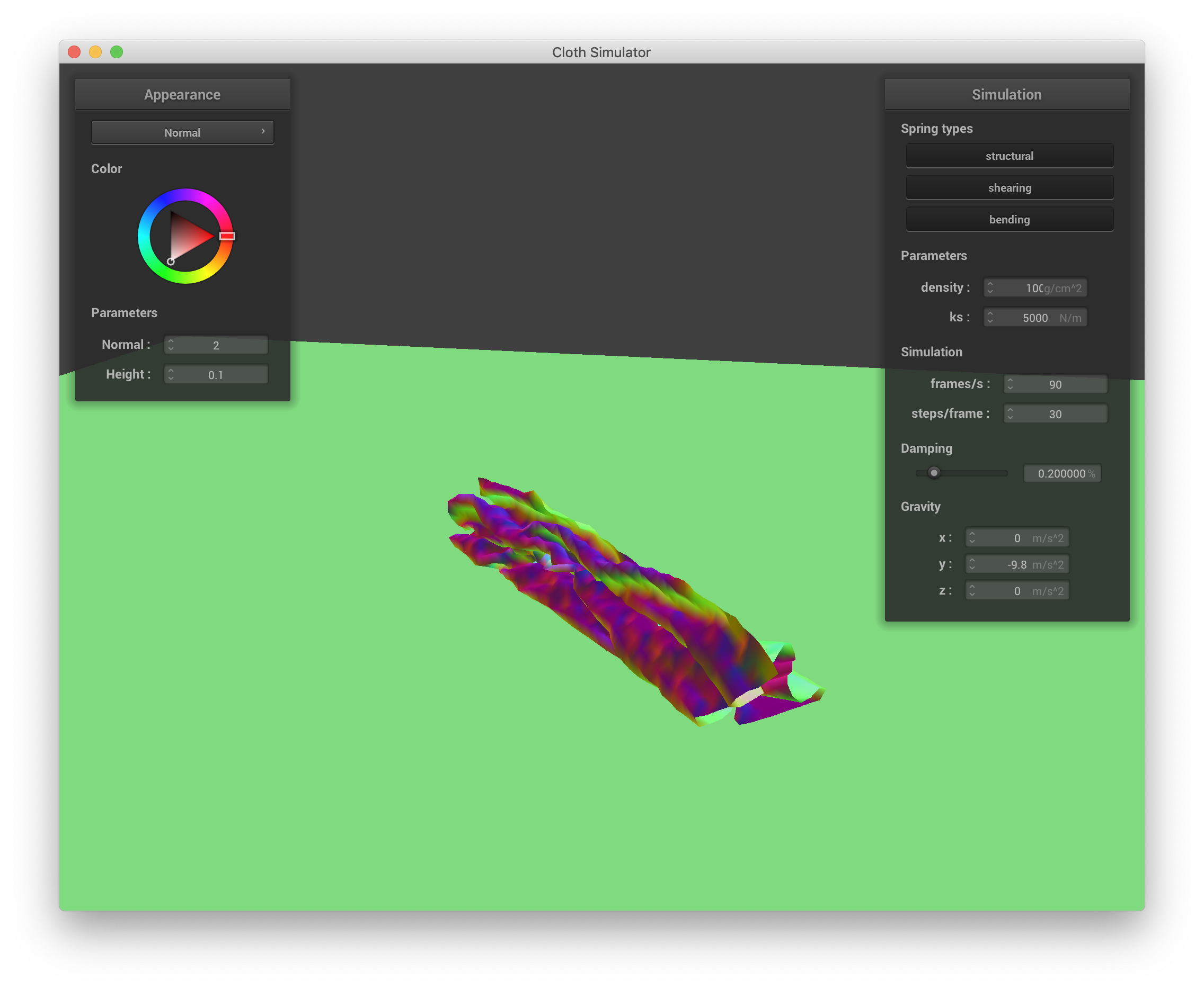
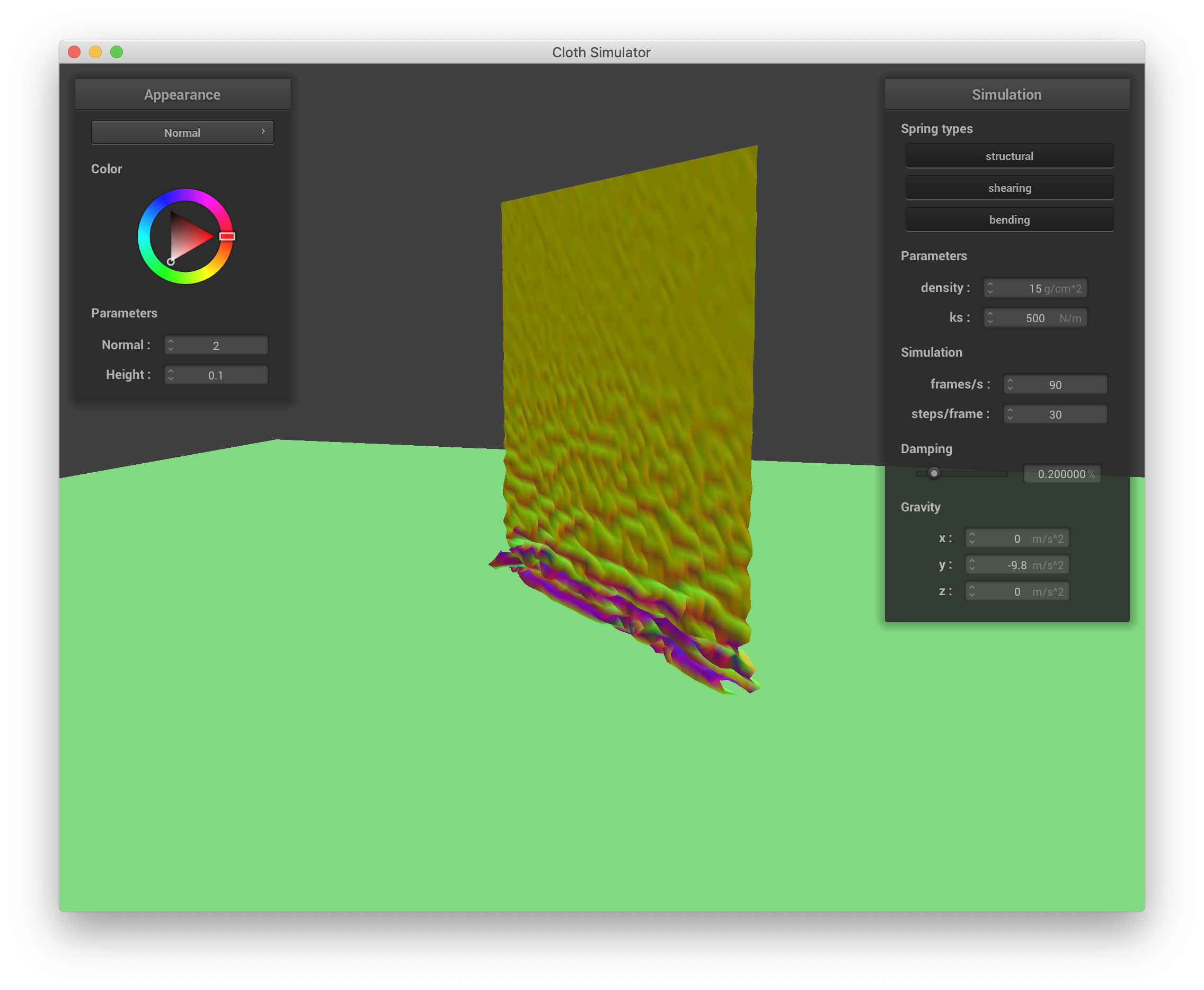
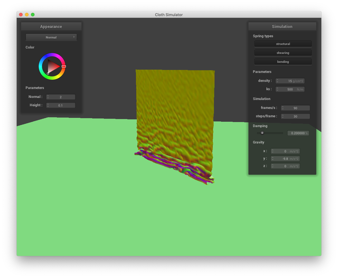
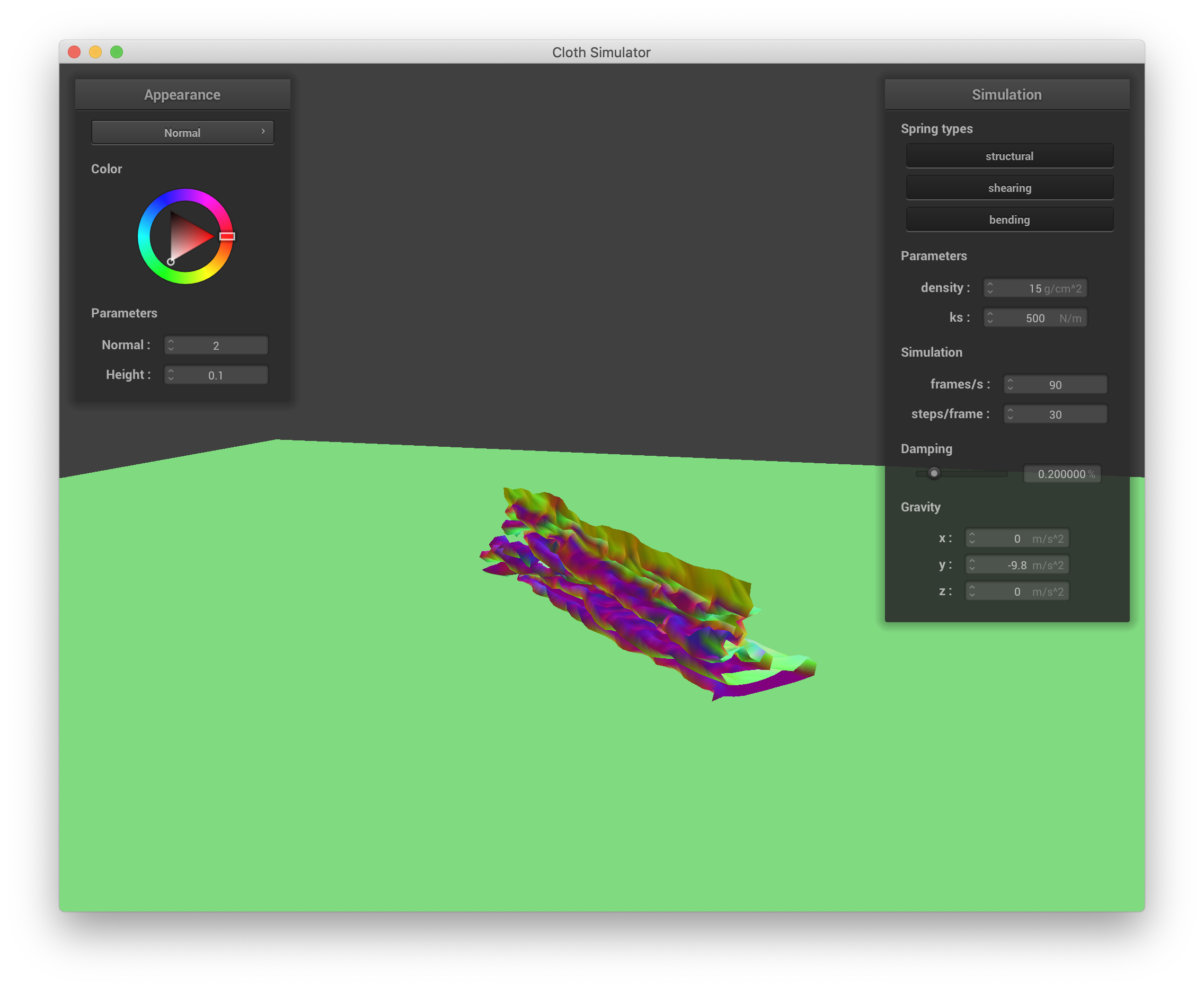
Self Collision with Density Variation
Low density
 Density of 1 gm/cm^2 Part 1
|
 Density of 1 gm/cm^2 Part 2
|
Density of 1 gm/cm^2 Part 3
High density
 Density of 100 gm/cm^2 Part 1
|
 Density of 100 gm/cm^2 Part 2
|
 Density of 100 gm/cm^2 Part 3
|
 Density of 100 gm/cm^2 Part 4
|
Density is directly related to the mass of the cloth. When density is low, the cloth can just float down, resulting in large,
gentle folds as seen above. When density is high, the weight of the cloth causes it to compress into itself, resulting in many folds in a
much smaller footprint than the low density case.
Self Collision with ks Variation
Low ks
 ks of 500 Part 1
|  ks of 500 Part 2
|
 ks of 500 Part 3
High ks
 ks of 50000 Part 1
|
 ks of 50000 Part 2
|
 ks of 50000 Part 3
|
 ks of 50000 Part 4
|
ks is a measure of how stiff the cloth is. Notice that when ks is low, the cloth is quite malleable
and has many
folds; however, when ks is high, the folds become much larger as the cloth tries to preserve its
original shape as much as it can, folding only in large segments when it finally has to.
Part V: Shaders
Shaders are special programs typically written to be parallelized on the GPU that can perform various steps in rasterization pipeline. In this project
we're taking a look at two in particular: vertex and fragment shaders. They perform per-vertex and per-fragment operations, respectively. The vertex shader
typically applies transformations to vertices, e.g., modifying their position or normals, and writes varyings for use by the fragment shader.
Post rasterization, the fragment shader takes the varyings provided by the vertex shader, e.g., the tangent and normal vectors, to determine lighting
and assign a color or map a texture to a given fragment. The full shader can be constructed
by compiling and linking the vertex and fragment shader together.
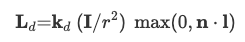
To start, diffuse shading for each fragment was implemented using the following equation:
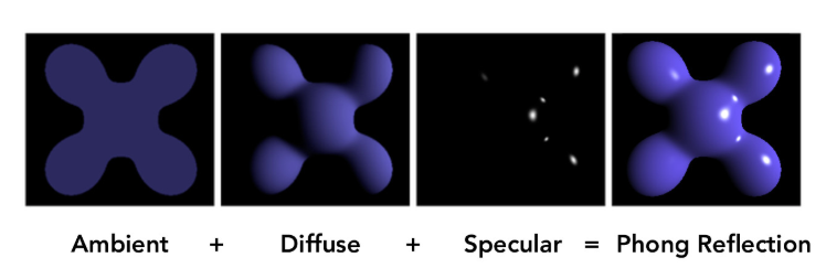
Blinn-Phong builds upon diffuse shading for each fragment by incorporating ambient and specular components to create a scene that depends on view direction. Specifically,
ambient shading is used to account for disregarded illumination and as a filler for black shadows, diffuse lighting
uses the normal to calculate additional view independent lighting, and finally specular shading is used to capture the view dependent effect by
increasing intensity along the mirror reflection direction of the lighting. Visually, the different components of Blinn-Phong can be seen below:
Mathematically Blinn-Phong can be modelled as follows:

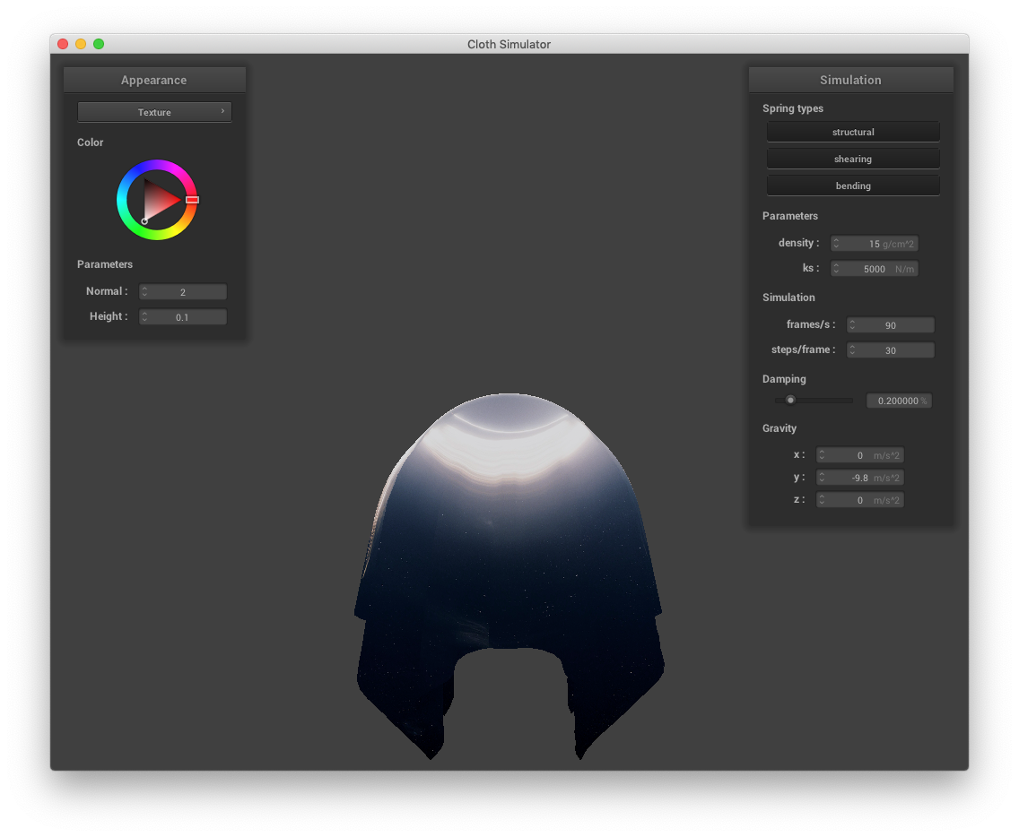
Texture mapping was implemented by simply calling the provided texture sampling function for each fragment.
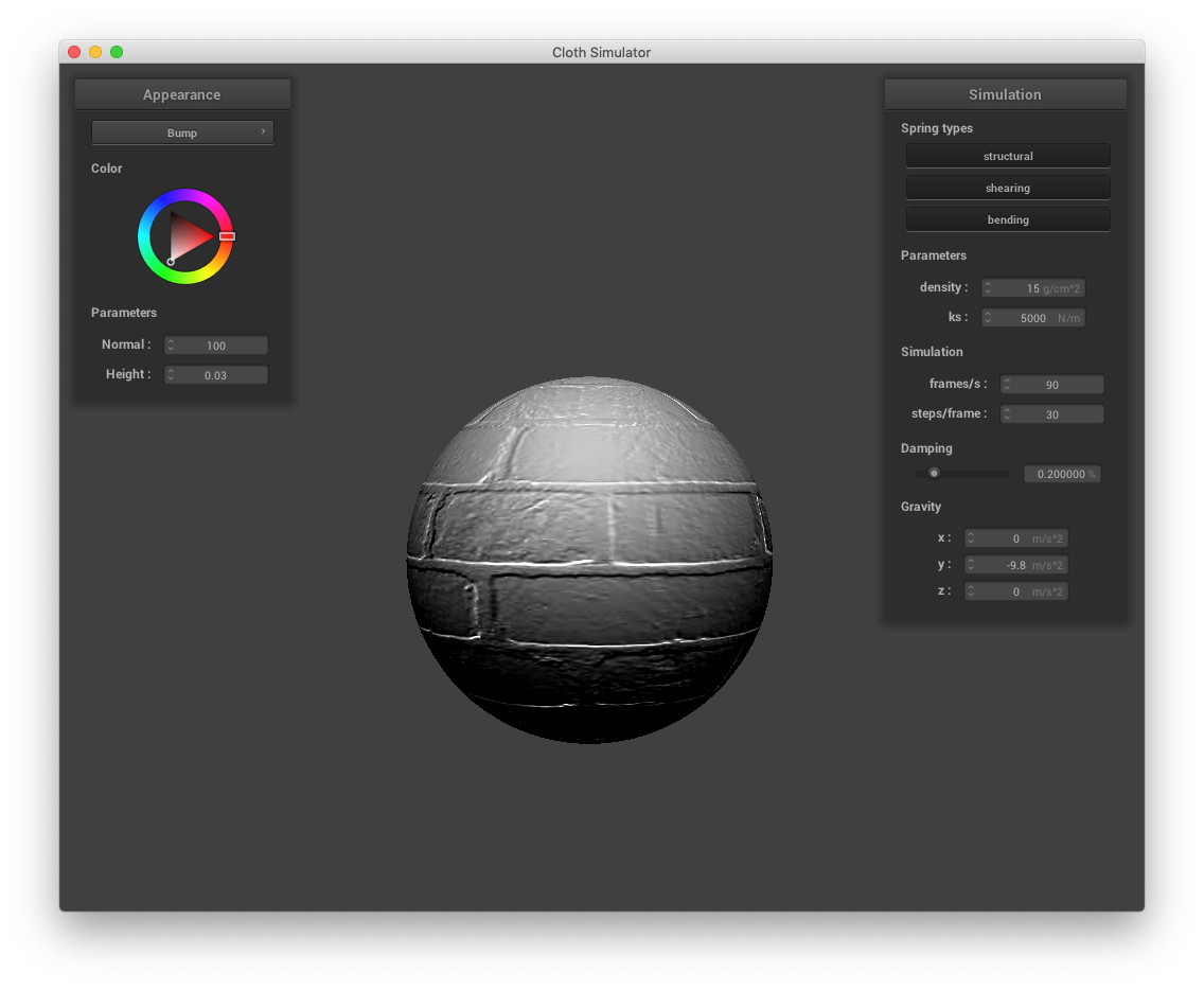
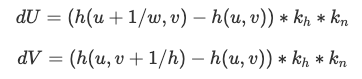
Bump mapping was slightly more involved, due to the need to calculate new displaced world normals for each fragment to give the illusion of detail such as bumps
on a given object. To do so, the following steps were taking:
- To start, dU and dV were calculated using:
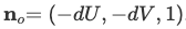
- Next the object space normal was calculated as such:
-
The conversion matrix from object world space was defined:
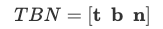 where
where

and t is the tangent vector.
- Finally, the displaced world space normal could be found using:

The displaced world space normal was then fed into the previously implemented Blinn-Phong model to get the bump mapped effect.
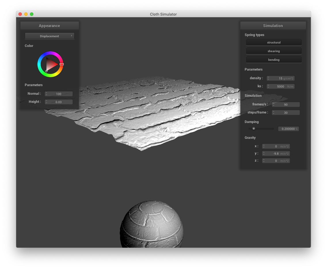
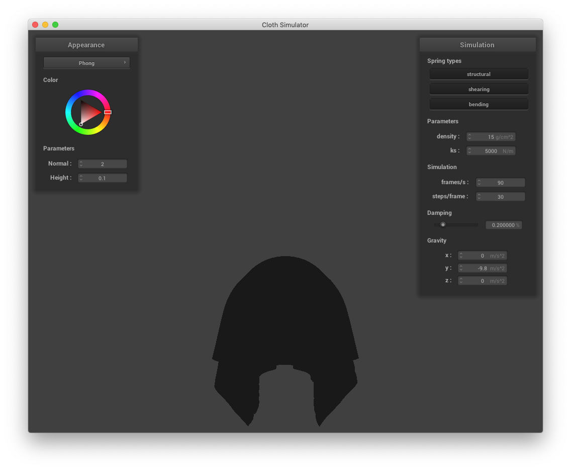
In addition to bump mapping, we also implemented displacement mapping, where instead of modifying normals to give the illusion of detail, we
physically manipulated the vertices themselves, calculating new positions using the following equation:
Finally, we implemented environment-mapped reflections, in which we sampled the texture to be mapped to the fragment using not just
the texture itself, but also the outgoing eye-ray reflected across the surface normal.
Screenshots
Blinn-Phong Decomposition
Ambient component only
 Diffuse component only
 Specular component only
 Entire Blinn-Phong model
Custom Texture
Bump Mapping vs Displacement Mapping
Sphere Coarseness Comparison (Bump vs Displacement)
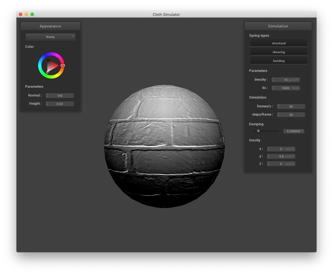 Bump mapping on
 -o 16 -a 16
|
 Bump mapping on
 -o 128 -a 128
|
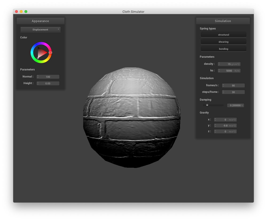 Displacement mapping on
 -o 16 -a 16
|
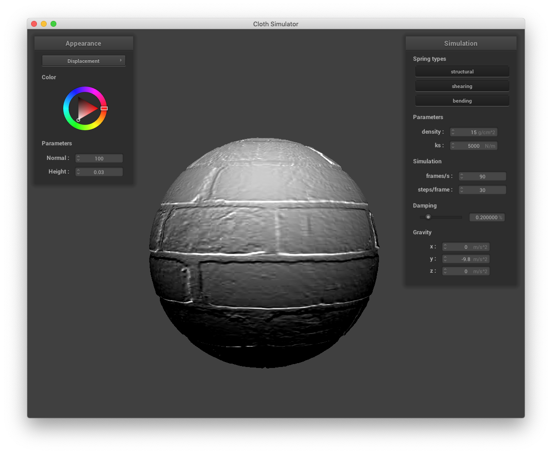 Displacement mapping on
 -o 128 -a 128
|
Variations in sphere coarseness don't impact bump mapping as much as they impact displacement mapping due to differences in
the nature of the
two mapping techniques. Whereas bump mapping doesn't fundamentally change the mesh of the object since we're just computing a temporary displaced normal to determine
fragment color, displacement mapping changes the vertices themselves, which is directly impacted by the granularity of the mesh.
Consequently, notice that there are minimal changes between the two bump mapping images--the sphere stays a sphere. However,
in displacement mapping, we can see a clear distinction between the low polygon-esque nature of the sphere using a coarse mesh ( -o 16 -a 16)
and the more nuanced divots between bricks using a fine mesh ( -o 128 -a 128). The difference in displacement mapping
is especially visible along the edge of the sphere, where the coarse mesh exhibits linear traits, whereas the fine mesh exhibits
more rounded ones.
Mirror Shader
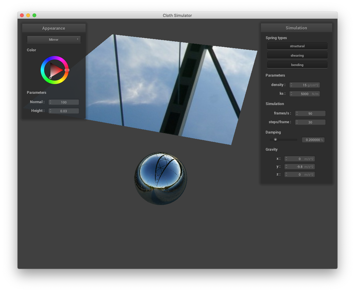 Overhead mirror shader
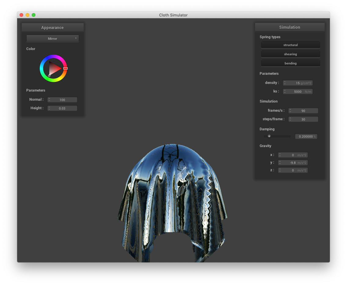 Mirror shader on cloth
|
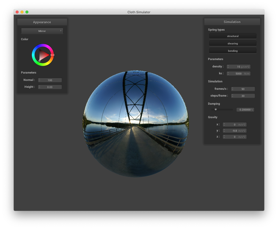 Mirror shader on sphere
|
Thank you for reading!
|